
A bench that measures photons, watts, and bits
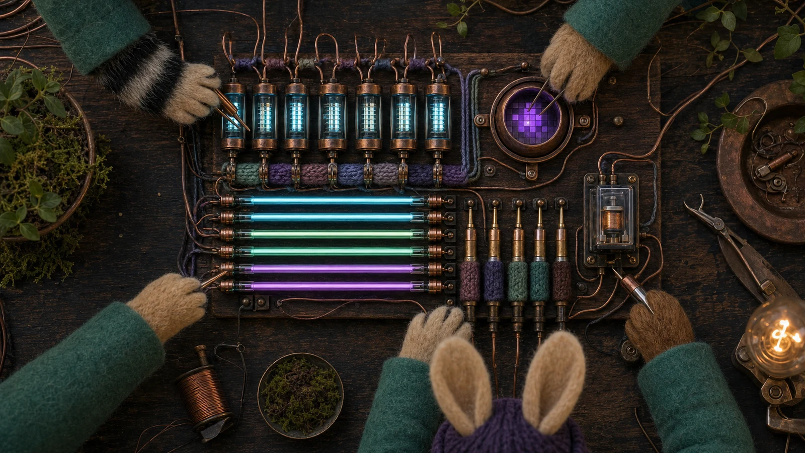
What we built to develop LED poles against: seven current monitors, a light sensor taped over one masked pixel, a logic analyzer on all six data lines, and a relay that can yank power from a Raspberry Pi on command. What each instrument is for, what the bench can answer that we could not ask before, and the numbers it produced in its first week.
Why build a bench at all
We build LED poles: steel tubes wrapped in six channels of double-row SK6813-mini strip, 480 pixels per channel, driven by an ESP32 taking 60 fps frames over Ethernet from a Raspberry Pi. Development used to happen against whichever pole happened to be standing in the shop.
A standing pole is good at exactly one question: does this look right. It cannot tell you how many watts a pattern draws, whether the wire is really carrying 60 frames a second, which of six channels is the one misbehaving, or whether the brightness you are looking at is the LED or the power limiter quietly rescaling everything.
Every question we actually care about is a measurement. So we built something to measure against: the same LED count as a real pole, laid flat on one surface where every pixel is visible at once, with the instruments wired in permanently rather than clipped on for an afternoon.
Three classes of instrument
The bench measures in three different currencies, and the reason for all three is that each one is blind to what the others catch.
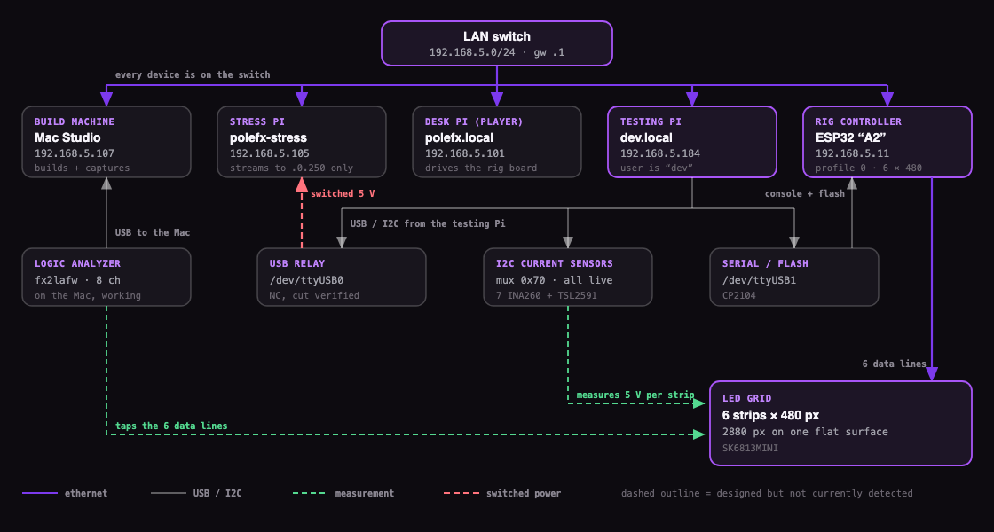
Watts. Seven INA260 current and voltage monitors on an I2C multiplexer. Six sit inline with each strip's 5 V feed. The seventh sits on the whole system's input.
Photons. A TSL2591 light sensor face-down over a single pixel with its neighbors masked off, so a single LED dominates the reading (measured below: 8,603 counts from the target, 5 from its nearest neighbor). It takes camera auto-exposure and human opinion out of brightness questions; gain, integration time and saturation still need managing.
Bits. A generic FX2 logic analyzer, eight channels at 8 MHz, clipped to all six LED data lines. The wire is the only place where "what the controller believes it sent" and "what the LEDs were actually told" are the same thing.
Then two pieces that are not instruments at all: a USB relay wired normally closed into a Pi's power lead, and a second Raspberry Pi whose only job is to be the thing that relay abuses.
Three currencies because a pattern can look correct while the wire runs at 42 fps. Power can sit exactly in spec while one strip is dark. A frame rate can be perfect while the pixels carry the wrong colors. Any single instrument will happily confirm that a system is healthy in the one dimension it can see.
The measurement that makes the rest trustworthy
Six current sensors give you six numbers. Nothing about six numbers tells you whether they are right.
The seventh is what makes them checkable. It sits on the system input, so the six strips should sum to it, less whatever the ESP32 and the board draw. Running normally:
six strips summed     6,816 mA
system input          6,948 mA
unaccounted             132 mA   (1.9%)
The six strips also agree with each other to within 12 mA. That closure is the bench checking itself, and it runs continuously rather than as a commissioning step. If a shunt drifts or a connector starts to fail, the gap opens and we see it without going looking. Its limits are worth stating: it catches single-channel and wiring failures, not a drift shared by all seven sensors, and agreement at one load point is a sanity check, not a calibration.
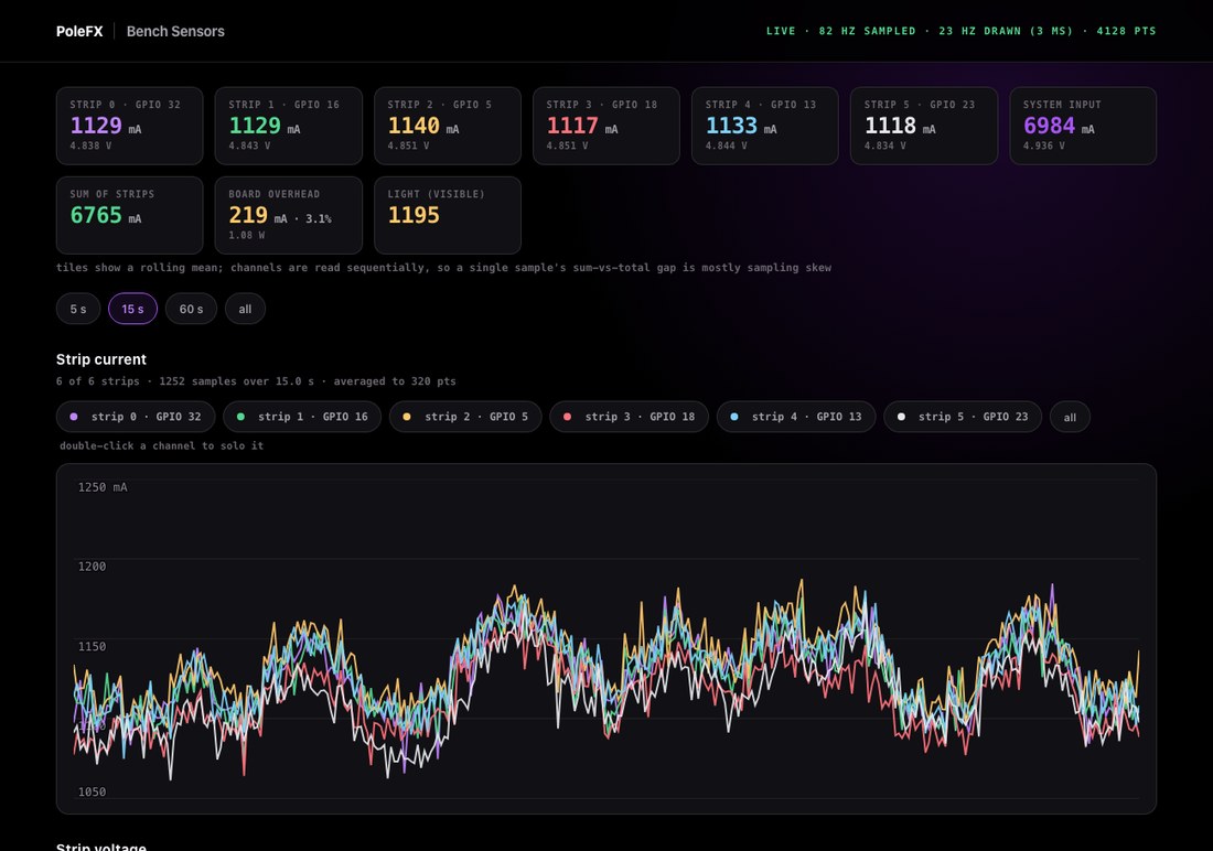
Those numbers come from one static frame held on the strips. On the live dashboard, with a pattern moving, the smoothed board-overhead trace (the ESP32 and everything else on the board) sits nearer 225 mA, about 1.1 W. That is a different operating condition, not the same residual, and the seven sensors are read sequentially, so any single instantaneous sample of the difference swings about 150 mA either way. The values to trust are windowed means, which is what both figures are.
The voltage side is quieter but useful. The input rail sits at 4.954 V while the strips read 4.853 to 4.869 V, so there is a consistent 90 mV of drop into the strips, and they track each other within 16 mV.
Knowing which strip is which
None of this helps if you cannot say which physical strip a reading belongs to. So we measured the wiring instead of assuming it: light one 480-pixel block at a time and read all three instrument classes together.
Each block raised exactly one current sensor by about 3.5 A and exactly one analyzer channel by about ten points of duty cycle, with everything else flat. Six measurements produce the whole map:
| pixels | firmware strip | GPIO | current sensor | analyzer |
|---|---|---|---|---|
| 0 to 479 | 0 | 32 | mux ch3 | D7 |
| 480 to 959 | 1 | 16 | mux ch2 | D6 |
| 960 to 1439 | 2 | 5 | mux ch1 | D4 |
| 1440 to 1919 | 3 | 18 | mux ch5 | D3 |
| 1920 to 2399 | 4 | 13 | mux ch6 | D2 |
| 2400 to 2879 | 5 | 23 | mux ch7 | D5 |
Neither the sensor order nor the analyzer order follows the strip order, and they do not follow each other. There was no pattern available to guess, which is the argument for measuring it once and writing it down.
The same sweep placed the light sensor exactly: pixel 0 of strip 0. Lit alone, that pixel reads 8,603 on the sensor's visible channel. Its neighbor reads 5. The one after that reads 0. The masking works.
One technique from that sweep is worth passing on. To find which analyzer channel carries a lit strip, you cannot ask whether a channel is active. A dark strip still clocks every bit of every pixel, so all six channels always look busy and their edge counts are identical by design. What moves is duty cycle: all-zero data sits near 20%, every bit being a 250 ns pulse in a 1.25 µs period, and climbs from there as bits turn on.
What the bench can now answer
Is the pole really at 60 fps? Not according to a counter in the firmware, which can only report what the firmware believes. Off the wire: 1.25 µs bit period, pulse widths in two clean classes at 250 and 750 ns, and 60.0 frames per second on all six data lines. Being off the wire is what matters, because our own tooling has a known habit of reading 58.8 for a true 60.0. Six lanes is not six trials, though: all six outputs come from one I2S engine and their frame starts agree to within a sample, so what six lanes buy is a check that no lane is missing frames, not six independent frame rates.
What is this pattern drawing, per strip, right now? Live, from a sampler polling at about 170 Hz, with the running total and the sum-versus-total gap beside it.
Am I looking at the LED or at the power limiter? This is the most useful
thing the light sensor has told us so far. The firmware runs
FastLED.setMaxPowerInMilliWatts(30000), and when the estimate crosses that
ceiling FastLED rescales the entire frame uniformly. Hold pixel 0 lit and add
company around it:
| lit pixels | strip mA | system mA | pixel 0 brightness |
|---|---|---|---|
| 1 | 389 | 2340 | 100% |
| 60 | 2522 | 4450 | 99% |
| 120 | 3599 | 5481 | 75% |
| 240 | 4094 | 5985 | 46% |
| 480 | 4438 | 6332 | 26% |
The brightness column is the sensor's raw visible-channel count as a fraction of the one-pixel reading. Same pixel, same white, same geometry throughout, so the sensor's spectral response cancels out of the ratio and only its linearity has to hold.
Pixel 0 never changed. The tell is that current plateaus while brightness falls: 240 to 480 lit pixels adds 8% more current and halves the brightness. One sweep, five points, so what it pins down is that the knee is somewhere between 60 and 120 lit pixels, around 27 W measured against a 30 W setting.
Knowing that is the difference between a useful optical bench and a misleading one. Above roughly a hundred lit pixels the light sensor measures the limiter rather than the LED, so optical comparisons stay below the knee, or we raise the ceiling for the duration of the measurement.
Can we finally test whether yanking power corrupts the SD card? We ship read-only root filesystems with a tmpfs overlay specifically so that pulling the plug cannot corrupt anything, and we believed that without ever having tested it at volume. The relay makes it testable: energize to cut, release to restore. The victim Pi drops off the network 2.0 seconds after the cut and is back 24.1 seconds after the restore, which is now the boot-to-network baseline.
One cycle is not evidence, but the check is automatable: after each cycle,
git fsck the application repo, look for ext4 errors in the kernel log, and
confirm the data partition still reports clean. The first cycle came back clean
on all three.
The dashboard
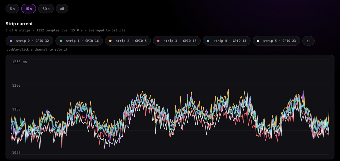
Everything above streams live to a page served from the bench Pi itself, on the shop LAN. Six strip currents with per-channel solo and mute, strip voltage against the input rail, the sum-versus-total cross-check, board overhead, and the light sensor, over a 5, 15 or 60 second window.
Two things about building it were more interesting than expected.
The sampler was slow for a reason we had backwards. It ran at 7 Hz, and the obvious suspect was the sensors' on-chip averaging. Benchmarking said otherwise: averaging made no measurable difference to read throughput at 64, 16 or 1. The INA260 converts continuously in the background, so a read just fetches the last result and the entire cost is I2C transactions. (The averaging setting still matters to the measurement itself, setting the conversion window and how independent successive samples are; it just was not what made reads slow.) The fix was the bus clock:
| bus clock | 7 sensors, current + voltage | current only |
|---|---|---|
| 100 kHz | 34.8 Hz | 69.7 Hz |
| 400 kHz | 103.6 Hz | 213.5 Hz |
We stop at 400 kHz because the light sensor is only rated that far, not because the wiring gave out; what the bus itself could carry is untested. With voltage refreshed every tenth pass and light on its own 120 ms timer, since that part needs 100 ms to integrate and reading it faster returns the same number, the sampler now polls at about 170 Hz. Poll rate, not information rate: with the four-sample averaging we run, a fresh current-and-voltage conversion lands about every 8.8 ms, so roughly 114 Hz of the polls carry new data and the rest re-read the last conversion. The browser gets 25 coalesced updates a second. Three different rates, and conflating them is how sampling claims go wrong.
Polling was the wrong transport. A fixed poll interval forces a choice between latency and request overhead; the page now pushes Server-Sent Events, batched at 25 Hz and coalesced onto animation frames.
A charting problem worth knowing about
Drawing 170 samples a second into a chart a thousand pixels wide means averaging them into buckets, and how you cut those buckets matters more than it sounds.
Cut them by array index, the obvious way, and every new sample changes the row count, which shifts every boundary, which lands a measurement that will never be taken again in a different bucket on the next frame. The plotted value moves. The data is static and the chart is not, and the result reads as noisy sensors.
Anchor the bucket edges to absolute time instead and a sample falls in the same bin for its whole life, so the chart advances by whole bins.
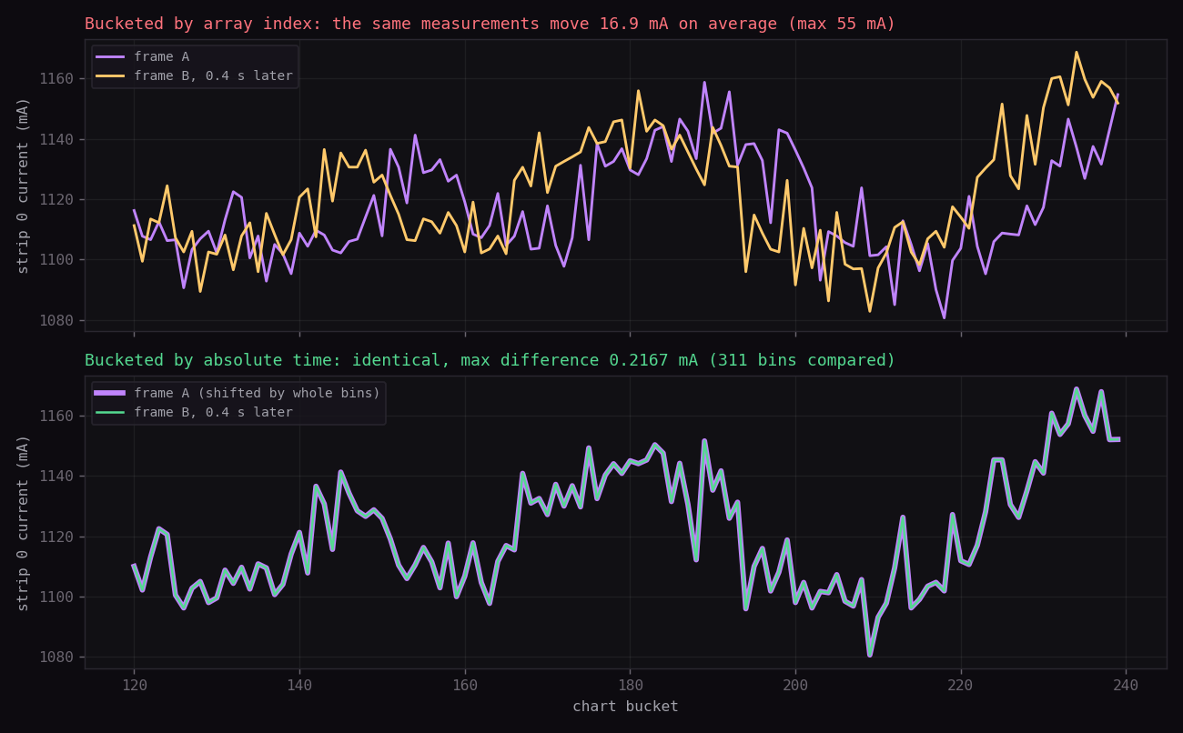
Same data, two frames 0.4 seconds apart. Bucketed by index, the same measurements move 16.9 mA on average and up to 55 mA. Anchored to time, the bins that overlap are identical to four decimal places.
The same thought applies one layer up. The y-axis was recomputing its extremes every frame, so a single new sample shifted the whole scale. Ranges now snap to round steps and only move when the data would actually clip.
There is one more place the presentation does real work. The board overhead chart draws the raw per-sample difference faintly behind a smoothed line, because the seven sensors are read sequentially while the pattern is moving. A single sample's difference swings 150 mA around a value that is genuinely steady. Plotted raw and alone, it would look like the controller was unstable.
Capturing the wire on demand
The analyzer gets its own panel, and deliberately not a live view. Eight channels at 8 MHz is 8 MB/s. That is not something to stream at a browser, and at any readable zoom a scrolling waveform shows either a solid block or three bits out of 11,520. It is a burst instrument.
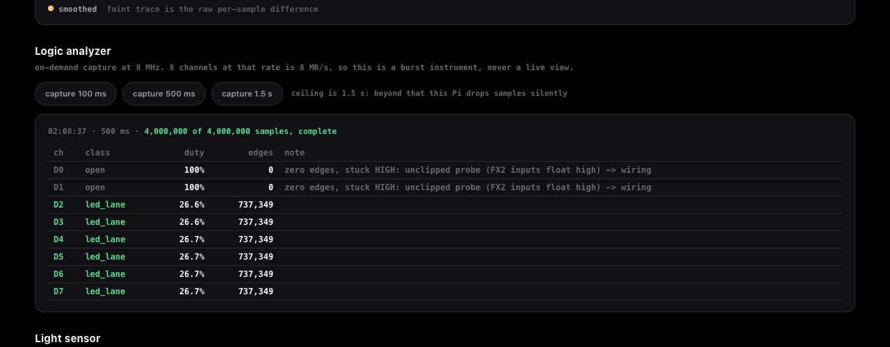
A button takes a capture, decodes it with the same tooling our bench scripts already use, and reports what each channel is: an LED lane, an unclipped probe floating high, or a probe that has come loose.
The interesting part is the guard. This Pi sustains 8 MHz cleanly to about 1.5 seconds. Ask for two and it loses 10 to 16% of the samples, and it does so silently: sigrok returns success, and the frame rate decoded from the truncated data still reads 59.9. Exactly the sort of number that gets written down and believed.
So the panel compares the returned sample count against what it asked for, and any shortfall voids the capture rather than reporting figures derived from a gap. We tested that by deliberately asking for 2.5 seconds: 33.7% lost, correctly refused, no numbers shown.
Decoding the wire in the browser
The panel tells you what each channel is. The scope tells you what it
said. Every capture is addressable at /scope, which pulls the raw
binary and decodes it client-side.
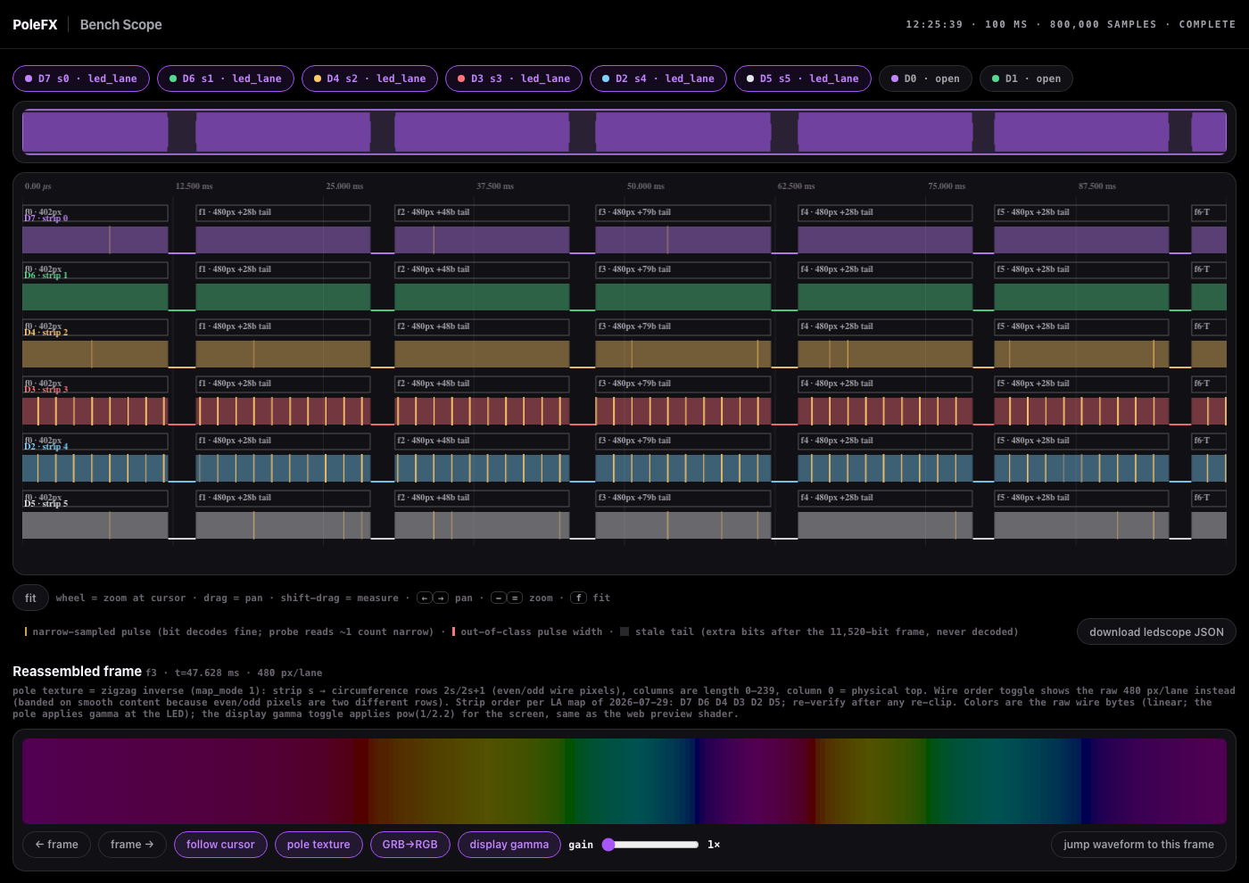
Lanes are labeled by physical strip rather than by probe number, using the
map from earlier, so D7 · strip 0 reads the way you think about the
hardware instead of the way the clips happen to sit. Each frame is annotated
with how many pixels it carried, and the whole capture has a minimap above it
for navigation.
Two things fall out of that annotation immediately. The first frame in this
capture reads f0 · 402px, because the capture started partway through it.
And every complete frame in this capture carries a stale tail: +28b,
+48b, +79b. Those are extra bits arriving after the 11,520 that make up a
frame. They are never decoded into pixels, and now they are visible rather than
theoretical. How long the tail runs is a separate question from whether it is
there, and this capture is far too short to answer it.
Zoom in and the decode goes all the way down:
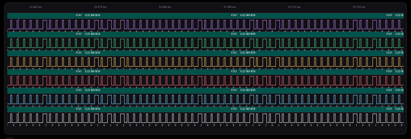
Every pulse carries its decoded bit underneath, and pixel boundaries are
marked with the color that pixel was told to be: #241 G21 R0 B16, then
#242 G21 R0 B18. That is the byte order as it exists on the wire, green
first, which is why the viewer has a GRB→RGB toggle rather than silently
reordering it.
Below the waveform the frame is reassembled into the pole's actual texture,
which means unpicking the zigzag mapping: strip s becomes circumference
rows 2s and 2s+1, with even and odd wire pixels landing on different rows,
and column 0 is the physical top of the pole. There is a toggle to see the raw
480 pixels per lane instead, which looks banded on smooth content precisely
because adjacent wire pixels are not adjacent in space.
The colors are the bytes as they physically left the controller, which means
after the firmware's mapping, gamma, brightness and power-limit stages: they
are everything the LED will be told, not necessarily what the source frame
said. On this bench board gamma is 1.0 and the test content sits below the
limiter knee, so the bytes happen to pass through linear; a production capture
will not numerically match source frames without accounting for those stages.
A separate display-gamma toggle applies pow(1/2.2) for the screen, matching
the web preview shader, so what you compare against is the same transform the
preview uses rather than an ad-hoc one.
Captures export as LEDscope JSON, which keeps the existing replay viewer as the place to watch a capture as an animation rather than duplicating it here.
What it costs, and what is next
Roughly $130 of sensors on a STEMMA QT chain and a USB relay, all bought for the bench, plus three Raspberry Pis pulled from the box of pole stock, two of which exist only to be measured or abused.
The analyzer is the cheapest thing on the bench by a wide margin. These FX2 clones go for about $3 on Alibaba, or $6 to $12 on Amazon if you would rather have it this week. For that you get eight channels at 8 MHz, which is enough to decode every bit of every pixel of every frame on all six data lines at once. It is comfortably the highest ratio of answered questions to dollars of anything here.
The sensor suite and the analyzer each have their own post: the power and brownout measurements and chasing 60 fps down the LED wire.
Next is automation. Every number above was produced by a human deciding to go and look. The instruments are now reachable from one machine, on one page, with the maps written down and the traps documented, which is the state where a nightly run can start doing the looking instead.
Every number in this post is read off an instrument on the bench described, over 2026-07-28 and 2026-07-29, except the 8.8 ms conversion interval and the 114 Hz that follows from it, which are arithmetic on the sensor configuration. The dashboard video and the bucketing figure are captures of live data, not reconstructions.