
Measuring an LED pole until it browns out (on purpose)

Real current, voltage, and light measurements from an SK6813 LED installation: what FastLED's power limiter actually delivers, a per-pixel power model that tracked whole-pole draw within 3%, and a deliberately induced power supply collapse.
Why
We build LED poles: steel tubes wrapped in six channels of double-row SK6813-mini strip (480 pixels per channel, 2,880 pixels per pole) driven by an ESP32 receiving frames over Ethernet at 60 fps from a Raspberry Pi.
Our worst field failure mode is ESP32 brownout. If the LEDs demand more
current than the supply can deliver, the 5 V rail sags, the ESP32's brownout
detector fires, and the controller reboots mid-show. The firmware defends
against this with FastLED's power limiter,
FastLED.setMaxPowerInMilliWatts(30000), but we had reasons to distrust that
number: FastLED estimates power from a generic per-LED model, and anecdotally
the pole "safely drew 42 W for weeks" with a 30 W setting.
So we built a measurement bench and asked four questions:
- What does the FastLED limiter actually limit to?
- How much power does a pixel draw, per color channel, per byte value?
- Can we predict a whole pattern's power from its pixels?
- What does the failure actually look like, and can we make it happen on demand?
The bench
A dedicated Raspberry Pi 4 reads seven I2C sensors through a PCA9548 multiplexer:
- 6x INA260 precision current/voltage/power monitors, one inline in each strip channel's 5 V feed;
- 1x TSL2591 light sensor taped face-down over a single LED, giving an objective optical measurement immune to camera auto-exposure.
Every board is a stock Adafruit part, about $130 the lot:
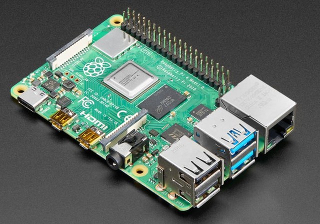
Raspberry Pi 4
bench hostRuns the capture scripts and generates the test frames. Separate from the pole's own controller.
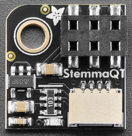
STEMMA QT breakout #6365
Pi header to QTPuts the Pi's I2C on a keyed 4-pin chain. Nothing to mis-seat, nothing to short.
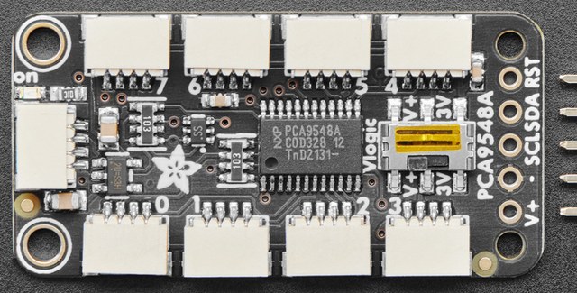
PCA9548 #5626
8-channel I2C muxEight switched I2C channels, so seven sensors that share one address can coexist.
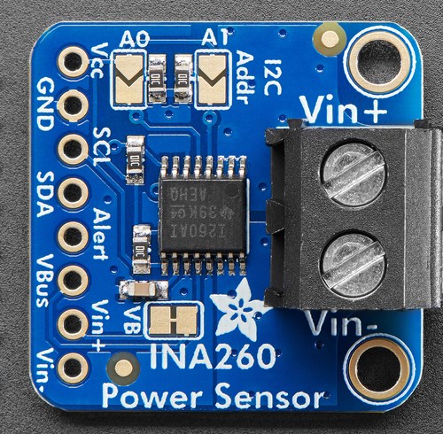
INA260 × 6 #4226
current, voltage, powerOne per LED channel, in series with its 5 V feed. Shunt and ADC are on-board.
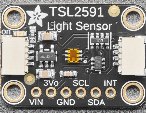
TSL2591 #1980
lightTaped face-down over one LED. Objective lux, immune to camera auto-exposure.
They wire into a STEMMA QT chain with the PCA9548 as the hub of a star: one cable per device, one mux channel per sensor, no address jumpers. The supply feeds the pole's controller and the controller feeds the strips, so each sensor is spliced into an output's 5 V wire: controller end into Vin+, strip end out of Vin−, on the screw terminals. Ground and LED data run straight through, untouched.
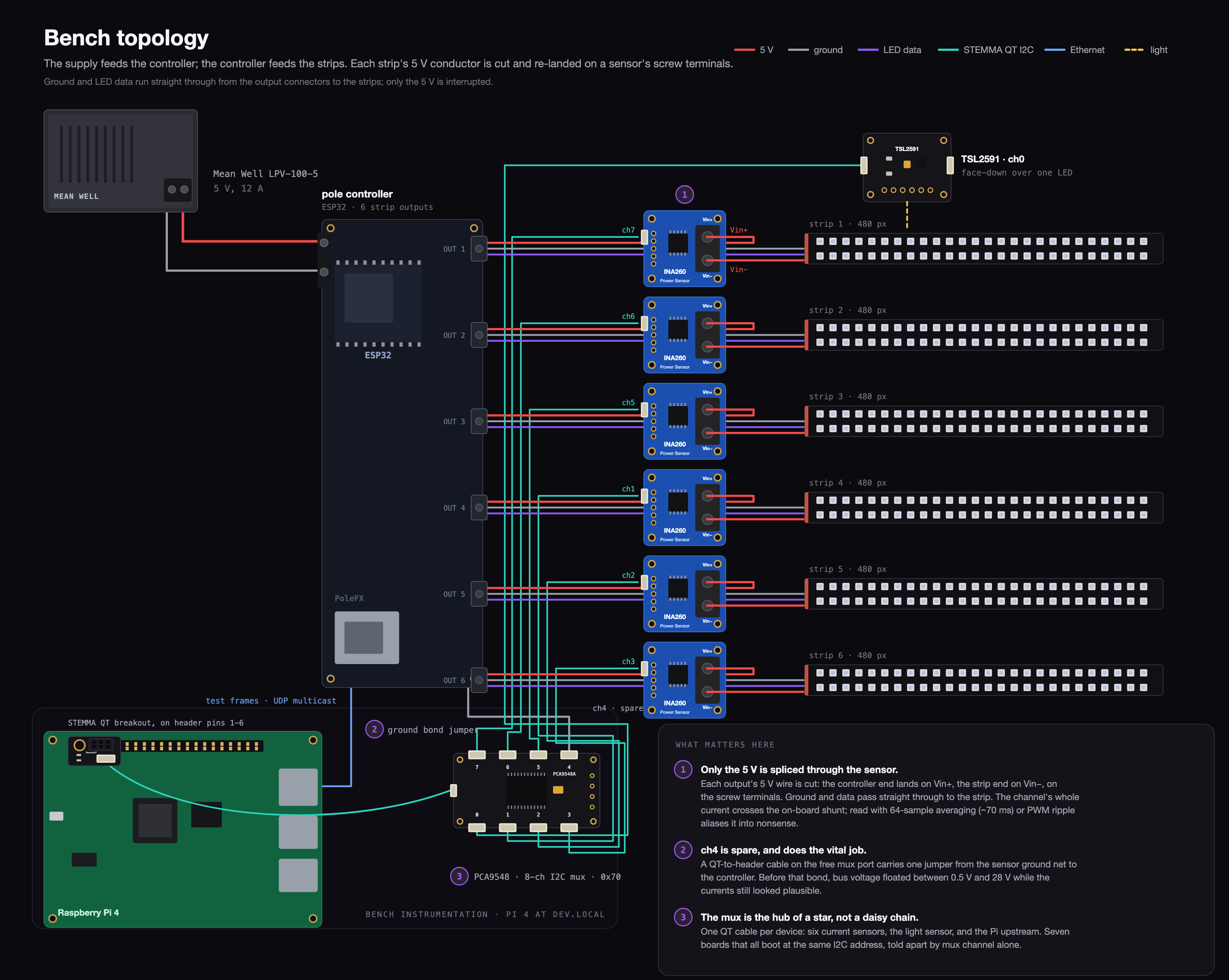
The pole under test is powered by a Mean Well LPV-100-5 (5 V, 12 A). Test frames were generated directly on the bench Pi and multicast to the controller in the pole's native UDP frame format, giving per-pixel control of all 2,880 pixels with no pattern engine in the loop. The ESP32's serial console and its heartbeat/alert broadcasts were logged throughout.
Two measurement gotchas worth passing on:
- A single INA260 conversion lies on PWM loads. SK6813 pixels chop their current at kHz rates, and 1.1 ms single-shot samples alias the ripple ringing on the supply leads: we measured "0 to 28.8 V" on a healthy 5 V rail. With 64-sample on-chip averaging (a ~70 ms window) the same rail reads 5.16 ± 0.33 V. Average everything.
- Bond your grounds. The sensor's bus-voltage measurement is referenced to its own GND pin. Until we ran one jumper from the PSU negative to the sensor chain, voltage readings floated between 0.5 V and 28 V while current readings stayed plausible, a nasty half-broken state.
Finding 1: a pixel's current is linear, and color doesn't matter
We drove a 60-pixel block through every byte value on each channel separately, measuring channel current with everything else dark.
Measured red, green, and blue current rises linearly with byte value at essentially the same slope; white is their sum.
Three results, all cleaner than we expected:
- Red, green, and blue draw identically: 48.0, 48.4, and 47.9 µA per pixel per byte-count. There is no "expensive channel" on this SK6813-mini batch, a common LED-strip folk belief that turns out not to apply here.
- White is additive: R+G+B predicts white within 1.4%.
- Current is linear in byte value from byte 8 to 255, with residuals under 0.1 mA. There is no gamma anywhere in this electrical path.
Those are electrical measurements, one strip's current sensor against the byte we sent, so they say nothing about how much light a watt buys on each channel.
On top of them sits a fixed cost. All six strips dark measure 2.08 A (10.4 W) for the whole pole, which is 0.72 mA per pixel. The lights-off tax is real.
The light output is linear too, on all four channels:
Measured red, green, blue, and white illuminance rises linearly with byte value, with no hidden gamma curve.
Lux tracks byte value point-for-point (byte 128 gives 0.509 of byte 255's output), and current is linear in byte value too, so within a channel the lux per amp is flat across the range at these timescales. The TSL2591 is photopically weighted, so this is not a statement that red, green, and blue turn watts into photons equally well; that needs a spectrometer, not a lux sensor. If your LEDs look nonlinear, that's your gamma table, not the silicon.
The pattern power model
Those two constants are the whole model. For a frame of RGB bytes:
current_mA = 0.72 x N_pixels + 0.048 x sum(every channel byte in the frame)
For our pole: I = 2.1 A + 0.048 mA x sum_of_all_bytes. Any pattern's power
can now be computed from its pixel data before it ever plays.
How good is it? Our first whole-pole validation run said "within 10-25%, over-predicting," and we had a tidy physical story ready (voltage starvation at the far end of each 480-pixel run). Then we noticed the trap: those measurements ran with the stock FastLED limiter armed, and FastLED's internal power estimate crosses its budget below the point where its hard clamp is obvious. The limiter was silently scaling frames we believed were clean.
With the limiter parked at 200 W, whole-pole measurements follow the per-pixel model. With the stock 30 W limiter, the same test is silently scaled.
Re-measured with the limiter parked at an unreachable 200 W, the whole-pole
curve tracks the per-pixel model within 3% up to 9.5 A, and the leftover
2-3% is honest rail sag. That is twelve points of uniform white between byte 2
and byte 18, not a survey of real patterns. Two lessons for the price of one:
the model predicts whole-pole draw closely where we checked it, and a power
limiter contaminates
measurements well below the point where you notice it clamping. If you are
characterizing LEDs behind FastLED, park max_power out of reach first or
your data quietly measures the limiter instead of the hardware.
Finding 2: what the FastLED limiter actually delivers
With the model in hand, we ramped a solid white frame while stepping
setMaxPowerInMilliWatts through 30 W, 45 W, and 60 W, rebooting between
settings. A detail worth knowing: FastLED only reads this value at boot.
A runtime change silently does nothing to the frame limiter until restart.
Limiter settings of 30, 45, and 60 W delivered 35.0, 46.0, and 56.1 W respectively.
Across the three settings we tried the measured clamp is linear in the setting, and nowhere near equal to it:
| setting | delivered (measured) |
|---|---|
| 30 W | 35.0 W |
| 45 W | 46.0 W |
| 60 W | 56.1 W |
delivered = 14.0 W + 0.70 x setting for this pole. Three points is not a linearity test, so the honest evidence for the line is the one held-out check: the middle point was measured after fitting the other two and landed within 1%.
The shape makes sense once you know FastLED's internals: its power model both overestimates per-pixel modulation draw (about 1.4x on SK6813-mini) and subtracts its own quiescent estimate from the budget, double-counting the idle draw. The two errors partially cancel near 50 W, which is presumably why nobody notices until they measure. The takeaway is not "FastLED is broken." It's that the setting is a knob, not a specification, and each LED type and count needs calibrating against measured watts, with a third point held back to check that a line is the right shape at all.
Finding 3: the failure is a cliff
Everything above happens in the safe zone. The real question was the failure.
First surprise: we couldn't brown it out with content alone at sane settings. With the limiter at 60 W, we hit the pole with 21 instant black-to-white steps (seven step sizes, three trials each) reaching 10.7 A measured, the worst dI/dt a pattern could ever produce. The rail never fell below 4.71 V, and 21 more steps delivered as a 100 ms ramp barely changed the dip. A properly calibrated limiter absorbed every content transient we could build; the supply's regulation, not the step rate, is what mattered.
At the stock 30 W setting the margin is even more decisive: five instant black-to-full-white steps (the worst frame any pattern can produce) held the rail at 4.87 V, drawing the calibrated 35 W. Five trials on one supply at shop temperature is not a proof of impossibility, but at the stock setting we could not get content anywhere near the edge.
So we raised the limiter beyond the supply's capability (100 W setting) and escalated:
A step to byte 32 holds the rail near five volts. A step to byte 40 collapses the supply.
- Byte 32 white: survives. The sensors measure 14.4 A sustained, 120% of the PSU's rating. The rail sags to 4.57 V and the Mean Well just delivers it, indefinitely.
- Byte 40 white: collapse, 3 for 3. The 18.7 A figure for this step is the per-pixel model's prediction, not a reading: once the supply folded the sensors saw 0.36 A, and nothing on the bench ever measured what the strips were asking for. The waveform is fascinating. The rail holds ~4.55 V for about 80 ms (the supply's overload timer riding through what it hopes is an inrush), then folds back to 1.6 V. The ESP32 browns out, the load vanishes, the supply recovers, the controller reboots: the exact field failure, reproduced on demand.
The supply survives repeated steps beyond its 12 A rating, then collapses to about 1.6 V at an estimated 18.7 A demand.
We never found a gradual danger zone, but we also never went looking inside the gap: "sustains 120% forever" and "collapses in 80 ms" are adjacent steps of our sweep, byte 32 and byte 40, and we swept nothing between them. So the transition is at most one step wide and might be much narrower or a little softer. What is clearly going on is two protection systems facing off: the supply's constant-current overload behavior versus the load's willingness to keep pulling.
The controller's own instrumentation confirmed each event: the firmware
counts brownout resets in RTC memory and broadcasts a PoleFX_alert line on
the network. Worth actually listening to; ours were being silently dropped
by the receiving server (fixed now).
What this means for brownout-proofing
What we concluded, in order of leverage:
- Calibrate the software limiter; it's the actual protection. Set
max_powerso the delivered watts (via the calibration line, not the setting) stay at or below the supply's rating. On this 60 W supply a setting of about 65 W delivers roughly 60 W; we run a 30 W setting (35 W delivered) for margin. With that in place, nothing we could throw at the pole, worst-case instant white included, got near the cliff. - Power the ESP32 through a buck-boost, not an LDO. Our collapse waveform shows the rail parking at 1.6 V during the fault. No 3.3 V LDO survives that, which is why the controller reboots rather than riding through and shedding load. A buck-boost is the right shape of answer, and we're planning the TPS63020, but be careful what it buys: TI specifies it down to 1.8 V of input, with undervoltage lockout at 1.4 to 1.6 V. Our floor is 1.62 V. So the part covers the 80 ms shoulder at 4.55 V and then sits below its own rated input exactly where the fault gets interesting, and whether it holds 3.3 V long enough for firmware to blank the strips is unresolved: it needs this waveform played into the real converter with the real controller load on it, not a part number. If it does stay up, a controller that survives collapse can blank the LEDs, kill the demand, and let the supply recover, turning a reboot loop into a one-frame flicker. That is the payoff we are chasing, not something we have measured.
- Per-output load switches (SY6288 or similar) close the loop. With the controller alive through faults, switchable outputs let it shed strips, stagger power-up inrush, and re-admit load gradually after a fault. Our step data says inrush from content isn't the killer, but staged re-admission after collapse is where the switches earn their place.
- Model your content if you bypass a limiter. The per-pixel model (0.72 mA/px + 48 µA/px/byte) predicted whole-pole white within 3% up to 9.5 A, which is as far as we checked it. We now compute worst-frame power for patterns at upload time.
Reproducing this
The whole bench is about $130 of sensors: INA260 breakouts on a STEMMA QT chain (no address jumpers needed, one I2C mux channel per sensor), a TSL2591 taped to an LED, and a Raspberry Pi. The most valuable habits: average over PWM ripple, bond the grounds once, verify every firmware reboot actually happened (lossy UDP config protocols will gaslight you), and let the failure happen. The collapse waveform taught us more than every safe measurement combined.
Data, scripts, and figures for this post were captured on a live bench in a
single evening. Currents, voltages, and lux are direct readings. Three numbers
are not: the 18.7 A at the fatal step is the per-pixel model's prediction for a
step nothing measured, delivered = 14.0 W + 0.70 x setting is a fit to three
limiter settings, and 0.72 mA per pixel is the measured whole-pole dark current
divided by 2,880.